How to use PostgreSQL for (military) geoanalytics tasks

03 Mar 2024

Geoanalytics is crucial in military affairs, as a significant portion of military data contains geoattributes. In this article, I will discuss how to use PostgreSQL to process geospatial data and address common geoanalytical tasks. The information will cover methods for finding the nearest objects, distance calculations, and using geospatial indexes to enhance these processes. We will also explore techniques for determining a point within a polygon and geospatial aggregation. The goal of this article is to provide practical examples and tips to enhance working with geospatial data and contribute to the development of new solutions.

The materials and data used in the article are open-source and have been approved by the military representatives.

First data source: how to import russian military polygon data into PostgreSQL

I will need certain datasets to initiate the analysis and showcase PostgreSQL's capabilities in geoanalytics. I decided to start with data on russian military facilities available on OpenStreetMap (OSM). The first step is to load this data into PostgreSQL, after which we can use tools to optimize queries and enhance their efficiency.

To import data on russian military objects from OSM, we will use the osm2pgsql tool. This open-source tool efficiently transfers data from OSM to PostgreSQL. We will load the russia-latest.osm.pbf file (3.4 GB) containing information about points, lines, roads, and polygons from OSM. After loading, the file will be used to populate the corresponding tables in PostgreSQL, where we can begin the analysis and processing of data.

The script we are using includes commands for loading OSM data, creating a new PostgreSQL database, and importing data using osm2pgsql:

After executing the script, five main tables will appear in our database:

osm2pgsql_properties—stores settings and properties used during the data import.
planet_osm_line—contains linear elements, such as roads and rivers.
planet_osm_point—includes point objects, such as buildings (not all buildings are marked as geographic polygons, so we will have to come up with something to be devised to work with these points).
planet_osm_polygon—stores polygons representing areas, such as military bases.
planet_osm_roads—stores transportation routes.

To simplify the analysis of military objects, we will create a table called military_geometries. The SQL script will select data from the planet_osm_line, planet_osm_point, planet_osm_polygon, and planet_osm_roads tables, filtering out military objects. A 100-meter buffer will be applied to lines, points, and roads using ST_Buffer. This will also allow us to create polygons based on points and lines, providing the ability to analyze, for example, whether a point is within the specified polygons.

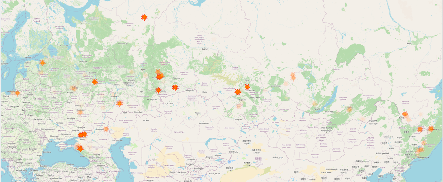
Executing the provided SQL script will allow us to create a military_geometries table that will contain polygons for 9,252 military objects identified on OSM:

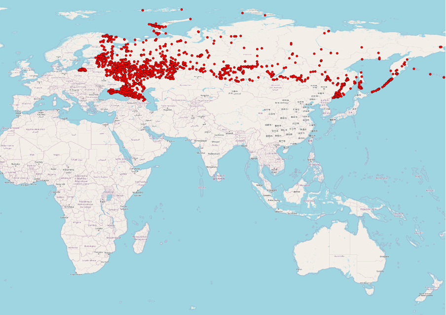Visualization of 9,252 military sites across russia and the temporarily occupied Autonomous Republic of Crimea using QGIS

In OSM, as in other open sources, information is subject to change. For example, from the beginning of 2022, 2,995 military objects in russia were deleted.

They say, "Screenshots don't burn", but such deletions often lead to the Streisand effect, where attempts to hide information only attract more attention. If you want to delve into the historical data of OSM and help identify such anomalies, you can use resources like GeoFabrik.de. Although this doesn't directly relate to our analysis, I want to show how these deleted objects look on a map, illustrating russian attempts to conceal essential data.

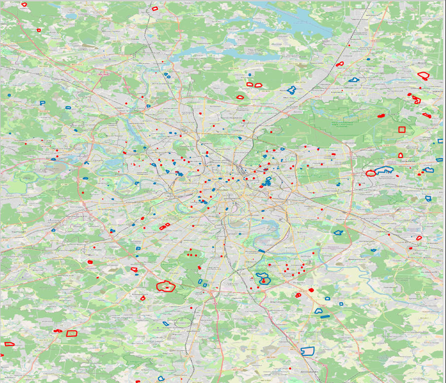Deleted after 01/01/2022 (blue) and existing (red) geographical polygons of military facilities in moscow

Second data source: fire data from NASA satellites

As the next data source, we will utilize information from the Fire Information for Resource Management System (FIRMS) developed at the University of Maryland with support from NASA and the UN in 2007. FIRMS allows real-time monitoring of active fires worldwide, utilizing data from Aqua and Terra satellites equipped with MODIS spectroradiometers and VIIRS on S-NPP and NOAA 20 satellites. The information is updated every three hours and even more frequently for the United States and Canada.

We will be using FIRMS data to identify fires within the territory of russian military facilities since 2022.

To download fire data from the FIRMS system, we will employ the following script, extracting all records of fires in russia from January 1, 2022, to the current date. These data will then be imported into a new table, viirs_fire_events, in the PostgreSQL database.

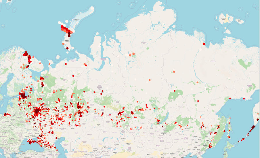
Therefore, we will populate the viirs_fire_events table, which will contain 1,711,475 records of fires in russia. These fires appear as follows:

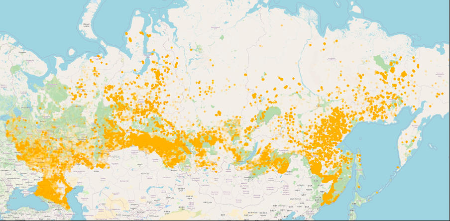Visualization of fires in russia since January 1, 2022 (1,711,475 fires)

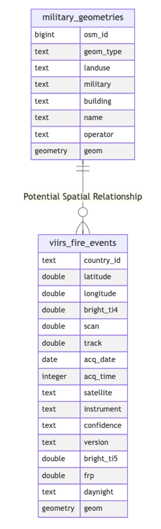
The viirs_fire_events table in the PostgreSQL database will be used to store detailed fire data, with fields for coordinates, satellite parameters, date and time of acquisition, and other critical metadata. A new column with a data type of GEOMETRY(POINT, 4326) will be automatically populated based on the data from the longitude and latitude columns.

Suppose you are interested in working with this data on military objects and fires, but the described process of extracting datasets seems time-consuming. In that case, there are exported CSV tables for you. You can download them via the following links: military_geometries, viirs_fire_events.

Searching for military facilities where fires occurred: points within the polygon

As for now, we have two tables: military_geometries and viirs_fire_events. Let's try to find those military facilities that have had fires (since the beginning of 2022) or those that have not yet 🙂.

Let's use an SQL query with the ST_Contains function to identify military objects where fires have been detected from NASA satellites.

As you've probably noticed, we've identified 129 military sites that have experienced fires since the start of 2022. What's intriguing is that, in some cases, these fires seem to have occurred more than once.

Military facilities where fires have occurred since the beginning of 2022 (the transparency of the facilities indicates the frequency of the fire incidents)

The second aspect you may have noticed is that the specified query took 54 minutes and 15 seconds to execute, which is quite long for such a straightforward operation. It's helpful to use the EXPLAIN ANALYZE command to understand the reasons for this duration. This command allows you to analyze the query execution process, identify potential bottlenecks, and further optimize the query to improve performance.

In this case, when using the Nested Loop Semi Join operator, we encountered a complexity of O(n*m), where n is 9,252 rows in the military_geometries table, and m is 1,711,475 rows in viirs_fire_events. This implies that each row from the first table is compared with every row from the second table, resulting in a huge number of operations.

Hence, let's discuss how we can speed up the execution of such a query by utilizing indexes.

Productivity boost: utilizing indexing in geoanalytics

PostgreSQL is renowned for its scalability features, offering numerous methods for accessing geospatial data within this database. To find all methods suitable for working with points in a two-dimensional space, we can execute the following query:

As a result, we will observe at least five access methods, including btree, hash, gist, brin, and spgist. I suggest investigating by creating indexes for each of these methods and operator classes. After creating the indexes, we will assess the query performance regarding fires at military facilities in russia to determine which methods are most effective for our task.

Index type	Index operator class	Filtering operator	Index creation time	Index size	Query execution time	Brief explanation
btree	btree_geometry_ops	There is no corresponding operator—the index is disregarded for this query.	1 sec 918 ms	81 MB	53 min 45 sec (129 rows affected)	Supports equality and range queries; retrieves data quickly and in an organized manner.
hash	hash_geometry_ops	There is no corresponding operator—the index is disregarded for this query.	3 secs 158 ms	59 MB	53 min 15 sec (129 rows affected)	Fast equality search; not suitable for ordering or range queries.
brin	brin_geometry_inclusion_ops_2d	@(geometry,geometry)	536 ms	0.032 MB	28 min 3 sec (129 rows affected)	Effective for large datasets with naturally ordered data; indexes block ranges rather than individual rows.
gist	gist_geometry_ops_2d	@(geometry,geometry)	11 secs 659 ms	94 MB	493 ms (129 rows affected)	Supports a wide range of queries, including spatial searches for overlap and proximity.
spgist	spgist_geometry_ops_2d	@(geometry,geometry)	6 secs 290 ms	78 MB	353 ms (129 rows affected)	Suitable for data with uneven distribution; supports a variety of split tree structures.
gist	point_ops	<@(point,polygon)	1 secs 426 ms	81 MB	306 ms (returned 132 records)	Perfect for point data; supports queries on spatial relationships, such as containment and intersection.
spgist	quad_point_ops	<@(point,box)	4 secs 849 ms	77 MB	243 ms (173 rows affected)	Utilizes quadtrees to index point data; effective in specific scenarios of spatial analysis.
spgist	kd_point_ops	<@(point,box)	5 secs 204 ms	93 MB	199 ms (173 rows affected)	Employs kd-trees for multidimensional point data; excellent for finding nearest neighbors.

Note: The operator classes mentioned do not utilize geometry data types for searching; they work with <@(point, polygon) and <@(point, box). As a result, the row counts may not match the output (for example, a complex geographic polygon may have been simplified to a rectangle).

The results table shows that the most effective indexes for our task are GiST and SP-GiST. Let's delve into how they operate.

How GiST works

Generalized Search Tree (GiST) indexes in PostgreSQL enable efficient sorting and searching across diverse data types using the concept of balanced trees. They provide the ability to develop custom operators for indexing, making GiST quite versatile and adaptive to specific requirements.

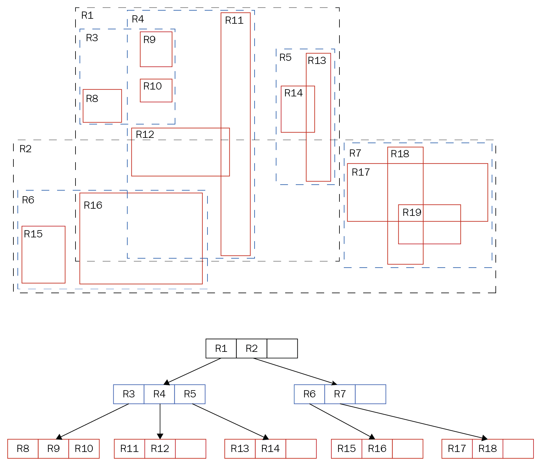The hierarchical structure of the GiST index in PostgreSQL [1]

In the example of a GiST tree depicted: at the top level, there are R1 and R2, serving as bounding boxes for other elements. R1 contains R3, R4, and R5, while R3, in turn, encompasses R8, R9, and R10. The GiST index has a hierarchical structure, allowing for significantly faster search. Unlike B-trees, GiST supports overlap operations and spatial relationship determination. This is why GiST is well-suited for indexing geometric data.

How SP-GiST works

Space Partitioning Generalized Search Tree (SP-GiST) indexes in PostgreSQL are designed for data structures that partition space into non-overlapping regions, such as quadrant trees or prefix trees. They enable the recursive division of data into subsets, forming unbalanced trees. This makes SP-GiST indexes particularly effective for in-memory usage, where they can quickly process queries due to fewer levels and small data groups in each node.

However, SP-GiST indexes have disadvantages when stored on disk due to the high number of disk operations required for their functioning, especially in large databases.

Considering this, GiST indexes often become a better choice, especially when working with polygons and complex spatial structures.

Finding the nearest neighbors: 10 fires near the Shahed production plant

Now, let's attempt to solve the task of finding nearest neighbors using PostgreSQL. Using our datasets, we will try to identify ten fires that occurred near the factory in russia, where Iranian Shahed drones are manufactured. For more detailed information about the plant, you can refer to the research conducted by the Molfar team. The factory is located in the special economic zone Alabuga in Tatarstan, where previously cat food and automotive glass were produced, and mushrooms were grown. However, after sanctions against Russia, its priorities shifted, and now it plays a key role in russia's plans for drone production.

One of the methods to solve this task is to create a buffer in the form of a circle around the selected target. This buffer is recursively expanded until the required number of results is obtained. In PostgreSQL, this can be implemented with the following SQL query, which forms the buffer and identifies fires that occurred within the specified radius from the selected object:

This approach involves gradually expanding the buffer and analyzing the results, which can be time-consuming.

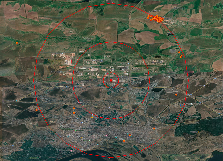A plant in Tatarstan that produces Shaheds with fire visualization within radii of 1.5 and 10 km

Various operators supported by GiST indexes can be utilized to optimize geospatial queries. To retrieve a list of available operators to use with a GiST index, you can execute an SQL query that scans the PostgreSQL system tables and provides information about operators associated with the gist_geometry_ops_2d operator class. This will help identify the most efficient operators for performing specific geospatial operations in the database.

Our GiST index provides extensive capabilities for working with geodata, allowing you to determine the spatial location of objects and measure distances. The <-> operator enables sorting objects by proximity to a specified point. In this example, we use this operator to identify the ten closest fires to the specified location.

The query turned out to be significantly faster—15 times swifter, compared to the previous methodology, and this is without repeated executions with a changed radius. We can analyze the query plan to confirm that the speed increased due to the use of an index and an operator. This way, we'll ensure that the index was indeed involved, which is the key to improving productivity.

As we can see, indexes, similar to GiST, extend analytical capabilities beyond simple comparisons, enabling the resolution of more complex tasks. As demonstrated in this article, open data can be effectively utilized for quickly assessing and defining goals on a global scale, including evaluating the success of target impact.

Uber's H3: a perspective on geospatial analytics and data aggregation

The H3, developed by Uber, is a hexagonal grid system designed to facilitate flexible and efficient distribution of geospatial data. It seems that H3 has the potential to become a common standard for working with geodata in the Armed Forces of Ukraine. Let's explore how this tool can be used for data aggregation and solving complex geoanalytical tasks.

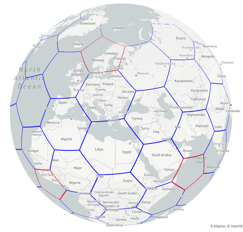Illustration of the Uber H3 hexagonal grid

As you can see in the image, each hexagon serves as a distinct geographic unit, simplifying the processing of intricate geoforms into uniform segments.

Level	Total number of objects	Number of hexagons	Number of pentagons
0	122	110	12
1	842	830	12
2	5,882	5,870	12
3	41,162	41,150	12
4	288,122	288,110	12
5	2,016,842	2,016,830	12
6	14,117,882	14,117,870	12
7	98,825,162	98,825,150	12
8	691,776,122	691,776,110	12
9	4,842,432,842	4,842,432,830	12
10	33,897,029,882	33,897,029,870	12
11	237,279,209,162	237,279,209,150	12
12	1,660,954,464,122	1,660,954,464,110	12
13	11,626,681,248,842	11,626,681,248,830	12
14	81,386,768,741,882	81,386,768,741,870	12
15	569,707,381,193,162	569,707,381,193,150	12

This is a hierarchical system consisting of 15 levels dividing the Earth's surface into hexagons. The zero level is divided into 122 sections, 12 of which are pentagons for accurately representing the Earth's spherical shape. We have approximately 569 trillion hexagons at the finest level, each representing a distinct geospatial object. The video below demonstrates how this works in practice. https://youtu.be/RbeYPqsFGPI

PostgreSQL can integrate H3 functionality through an additional extension. To install this extension, use the CREATE EXTENSION h3; command, and it is available on cloud computing services, including AWS RDS (my acknowledgments to AWS for their support of Ukraine). Once you've installed this extension, new functions become accessible. Let's explore those functions that might be useful for beginners:

Function	Input data	Output data	Description
h3_lat_lng_to_cell	latitude: FLOAT, longitude: FLOAT, resolution: INT	H3 index: BIGINT	Converts latitude and longitude coordinates into an H3 index at a specified resolution level.
h3_cell_to_boundary	H3 index: BIGINT	Array of boundary coordinates: GEOMETRY(POLYGON, 4326)	Transforms an H3 index into a geometric polygon representing the boundaries of a hexagon.
h3_get_resolution	H3 index: BIGINT	Resolution level: INT	Returns the resolution level of a given H3 index.
h3_cell_to_parent	H3 index: BIGINT, desired resolution: INT	Parent H3 index: BIGINT	Converts an H3 index into its parent index at a higher hierarchy level.
h3_cell_to_children	H3 index: BIGINT, desired resolution: INT	Array of child H3 indexes: SETOF BIGINT	Converts an H3 index into an array of child indices at a lower hierarchy level.
h3_polygon_to_cells	geometry: GEOMETRY, resolution: INT	Array of H3 indexes: SETOF BIGINT	Transforms a polygon into a set of H3 indices that fully or partially cover the polygon.
h3_grid_disk	H3 index: BIGINT, range: INT	Array of H3 indexes: SETOF BIGINT	Generates an array of H3 indices representing a hexagonal grid around the central H3 index, forming a “disk” of a defined radius.
h3_compact_cells	Array of H3 indexes: SETOF BIGINT	Array of compact H3 indexes: SETOF BIGINT	Consolidates an array of H3 indices, reducing the number of indices covering the same area.

To address the first task effectively, we can transform all our polygons into arrays of H3 indexes (hexagons) of a specified level. Similarly, we can process the centroids of fires by converting them into H3 indexes. By obtaining BIGINT data types for these H3 indexes, we can apply a standard B-tree index, which is particularly efficient in performing equality comparison operations. This will significantly improve query execution speed in complex geoanalysis tasks, ensuring fast and accurate results.

Let's examine a few simple H3 functions that will help better understand how this works in practice:


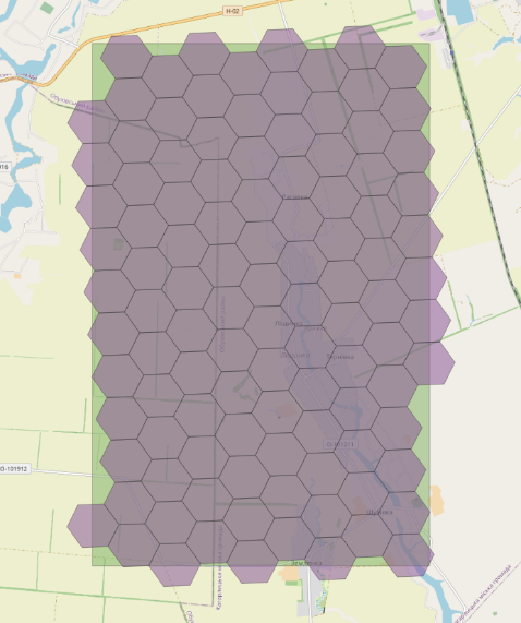
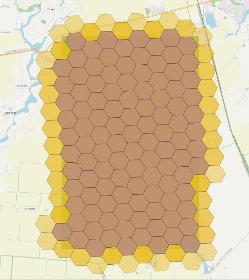
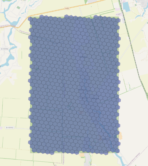
h3_polygon_to_cells(geom, 8) This function converts the geometry of a military polygon into a set of H3 indexes at the eighth level of resolution, effectively dividing the polygon into hexagons, each covering an area of 0.737327598 square kilometers, enabling detailed spatial analysis.	h3_grid_disk(h3_polygon_to_cells(geom, 8), 1) If certain areas of the polygon remain uncovered after applying h3_polygon_to_cells, you can use h3_grid_disk to create an additional ring of H3 indexes. It will expand coverage by adding hexagons around existing indexes, ensuring complete coverage of the defined geographic polygon.	h3_polygon_to_cells(geom, 9) Using the h3_polygon_to_cells function with a level 9 increases the grid’s resolution to a finer scale, where each hexagon represents an area of 0.105332513 square kilometers. This allows for greater accuracy in reproducing the geometry of the geographic polygon for detailed spatial analysis. However, it also results in more hexagons, which may negatively impact query execution speed.

During my presentation at PGConf.2023, the largest conference in Europe dedicated to PostgreSQL, I had the opportunity to showcase a series of more complex challenges that can be addressed by aggregating geospatial data using H3. One example involved the search for other drones located in the exact location and time, as well as the analysis of routes taken by drones traveling together, identified in different places over a specific period (Companion Analysis). You will have the opportunity to learn more about this topic in the continuation of this article. In the meantime, you can check out the materials of my presentation.

Within our datasets, we can analyze military objects and, through aggregation with H3, calculate the density of these objects in russia. The visualization of this analysis looks like this:

Visualization of the density of military objects in russia and the temporarily occupied Autonomous Republic of Crimea using H3 hexagons

Using H3 for aggregating geospatial data significantly enhances analytical capabilities, allowing for a more profound interpretation and visualization of complex spatial relationships.

Concluding remarks

If you are a representative of the Armed Forces of Ukraine and are seeking qualified support in the field of data, Big Data, or geoanalytics, feel free to reach out to me. My team of volunteers and I will gladly assist you with our knowledge and resources.

Additional resources I utilized in preparing this article:

While preparing this article, I used an Ubuntu server with the following characteristics and configured the PostgreSQL database as follows:

Taras Kloba's data engineering blog